6. Plotting#
- class Plotting#
Bases:
objectWORK IN PROGRESS
Holds many methods for plotting data in Scarabaeus.
Notes
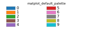
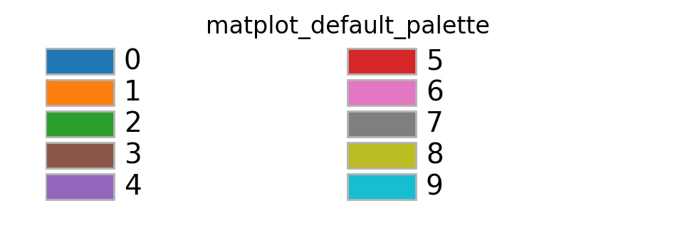
Scarabaeus’ plotting library contains multiple color palettes. See below for the colors contained within each:


Methods
apply_scale_to_axes([scale])Method to apply logarithmic or linear scaling to the axes of the plots.
compare_state_errors_norm(solution2, ...[, ...])Compares the state errors and sigma values of two solutions by plotting them together.
get_fig_handle(fig_handle[, show, save_dir, ...])Get the figure handle from another class
plot_asteroid_3d([obj_file, scale_factor, ...])Plot a 3D representation of an asteroid, either from an object file or a simple spherical mesh.
plot_compare_state_error_norm(...[, title, ...])Plots state errors norm for multiple iterations on the same figure for comparison.
plot_covariance(P_bplane_parameters[, title])Given a B-plane covariance, plot a graphical representation.
plot_covariance_est(n_sigma[, title, scale, ...])Plots the covariance history.
plot_gs_visibility(visibility_windows[, ...])Method to plot when the spacecraft can be seen by a set of ground stations
plot_measurement_availability(...[, scale, ...])Plots the availability of each measurement over time with x-axis labels as 'time - t_0' in integer days, where t_0 is the last time in combined_times.
plot_measurements_dataset(measurement_data)Method to plot the radiometric measurements as function of time.
plot_media_coverage([type])Plot DSN coverage intervals (in Ephemeris Time) from a media correction JSON file.
plot_multiple_covariance(sc_states, ...[, ...])Plot multiple covariances corresponding to different spacecraft positions and their covariances in the B-plane.
plot_multiple_orbits_3d(positions_list[, ...])Method for plotting multiple 3D trajectories, with default view as XY-plane.
plot_opnav_measurements(opnav_measurements)Method to plot opnav measurements as function of time.
plot_orbit_3d(positions[, title, origin, ...])Method for plotting a single 3D trajectory
plot_parameters_errors(true_trajectory, ...)Plots the state errors and sigma bounds for each component of parameters.
plot_parameters_errors_norm(true_trajectory, ...)Plots the state errors and sigma bounds for each component of parameters.
plot_parameters_estimate(epochs, n_sigma[, ...])Plots the estimated parameters over time with error bars and shaded uncertainty bounds (±nσ).
plot_position_velocity(data[, times, title, ...])Method to plot the position-velocity as function of time.
plot_postfits_asynchronous(dataset_names, ...)Plots the postfit residuals for various measurements (e.g., range, range rate, OpNav u, OpNav v) dynamically based on dataset names.
plot_postfits_asynchronous_with_hist(...[, ...])Plots postfit residuals with histograms for various measurement types.
plot_postfits_histogram(epochs, dataset_names)Plots the postfit residuals in a histogram for various measurements (e.g., range, range rate, OpNav u, OpNav v) dynamically based on dataset names.
plot_postfits_scatter(epochs, dataset_names)Plots the postfit residuals in a scatter plot for various measurements (e.g., range, range rate, OpNav u, OpNav v) dynamically based on dataset names.
plot_prefit_residuals(n_sigma[, title, ...])Plots the prefit residuals for range and range rate measurements.
plot_radiometric_measurements(...[, title, ...])Method to plot the radiometric measurements as function of time.
plot_scenario_param([scale, x_offset_flag])Plots the scenario paramters
plot_state_errors(true_trajectory, epochs, ...)Plots the state errors and sigma bounds for each component of position and velocity.
plot_state_errors_norm(true_trajectory, ...)Plots the state errors and sigma values over time.
plot_uv_measurements_over_time([scale, ...])Plot u vs v measurements, colored by time, and add subplots of u and v pixels over time with a semilog y-axis for the time.
plot_with_x_offset([x_offset_flag])Plot with an offset for x axis.
save_plot([save_dir, save_name, save_format])Method to save Plotting figures.
Method to seet custom styling for all plots within Plotting.
time_series_basic_line(time, data[, title, ...])Method for plotting time series data on a line plot.
time_series_basic_scatter(time, data[, ...])Method for plotting time series data on a scatter plot.
- static get_fig_handle(fig_handle, show: bool = False, save_dir: str = None, save_name: str = None, save_format: str = None)#
Get the figure handle from another class
- Parameters:
fig_handle (matplotlib plt.figure() object) – Figure handle generated outside the Plotting class
show (bool) – Option to show plot. Defaults to False.
save_dir (str) – Save directory. Defaults to None.
save_name (str) – Figure saving name. Defaults to None.
save_format (str) – Figure saving format. Can be “pickle” or “png”. Defaults to None.
- static plot_asteroid_3d(obj_file=None, scale_factor=1.0, ax=None, radius=None, name='Asteroid')#
Plot a 3D representation of an asteroid, either from an object file or a simple spherical mesh.
Parameters: - obj_file (str, optional): Path to the asteroid 3D model file (e.g., .obj). If not provided, a simple spherical mesh is plotted. - scale_factor (float): Scaling factor to adjust the size of the asteroid. Default is 1.0. - ax (matplotlib.axes._subplots.Axes3DSubplot, optional): 3D axes to plot the asteroid on. If not provided, a new figure is created. - radius (float, optional): Radius of the asteroid in kilometers if a simple spherical mesh is used. Default is None. - name (str, optional): Name of the asteroid to display in the legend. Default is “Asteroid”.
Returns: - ax: The 3D axes containing the plot.
Raises: - ValueError: If both obj_file and radius are None.
- static plot_gs_visibility(visibility_windows: dict, title: str = 'Ground Station Visibility Windows', epoch_start: str = None, show: bool = False, save_dir: str = None, save_name: str = None, save_format: str = None, scale: str = 'linxy')#
Method to plot when the spacecraft can be seen by a set of ground stations
- Parameters:
visibility_windows (dict) – dictionary of the GS visibilities
epoch_start (str) – Starting epoch
show (bool) – Option to show plot. Defaults to False.
save_dir (str) – Save directory. Defaults to None.
save_name (str) – Figure saving name. Defaults to None.
save_format (str) – Figure saving format. Can be “pickle” or “png”. Defaults to None.
scale (str) – Scaling option [‘logx’, ‘logy’, ‘logxy’, ‘linx’, ‘liny’, ‘linxy’]
- static plot_measurements_dataset(measurement_data, title: str = None, show: bool = False, save_dir: str = None, save_name: str = None, save_format: str = None)#
Method to plot the radiometric measurements as function of time.
- static plot_multiple_orbits_3d(positions_list, labels=None, origin=None, title: str = '@Sun, J2000', units: str = 'km', show: bool = False, save_dir: str = None, save_name: str = None, save_format: str = None, line_styles=None, colors=None, markers=None, view_xy_plane: bool = True)#
Method for plotting multiple 3D trajectories, with default view as XY-plane.
- Parameters:
positions_list (list) – list of several objects positions in X,Y,Z coordinates.
labels (list) – list of several objects labels. Defaults to None.
origin (np.array(,3)) – origin of the plot in X,Y,Z coordinates. Defaults to None.
title (str) – Title of plot. Defaults to “Reference Frame: J2000”.
units (str) – Units to use in the X,Y,Z labels. Defaults to “km”.
show (bool) – Option to show plot. Defaults to False.
save_dir (str) – Save directory. Defaults to None.
save_name (str) – Figure saving name. Defaults to None.
save_format (str) – Figure saving format. Defaults to None.
line_styles (list) – List of line styles for each orbit. Defaults to solid lines.
colors (list) – List of colors for each orbit. Defaults to default matplotlib colors.
markers (list) – List of markers for each orbit. Defaults to None (no markers).
view_xy_plane (bool) – Boolean to set the default view to XY-plane. Defaults to True.
- Returns:
Matplotlib figure object.
Method to plot opnav measurements as function of time.
- Parameters:
opnav_measurements (list[EpochArray,np.array,ArrayWFrame]) – Dictionary of the measurement, generated from the MeasurementDataSet
title (str) – Title of plot. Defaults to None.
show (bool) – Option to show plot. Defaults to False.
save_dir (str) – Save directory. Defaults to None.
save_name (str) – Figure saving name. Defaults to None.
save_format (str) – Figure saving format. Can be “pickle” or “png”. Defaults to None.
scale (str) – Scaling option [‘logx’, ‘logy’, ‘logxy’, ‘linx’, ‘liny’, ‘linxy’]
x_offset_flag (bool) – Offset value for X axis
- static plot_orbit_3d(positions, title: str = '3D Trajectory', origin=None, units: str = 'km', show: bool = False, save_dir: str = None, save_name: str = None, save_format: str = None)#
Method for plotting a single 3D trajectory
- Parameters:
positions (np.array(N,3)) – object position in X,Y,Z coordinates (no frame assuemd).
origin (np.array(,3)) – origin of the plot in X,Y,Z coordinates (no frame assumed). Defaults to None.
title (str) – Title of plot. Defaults to “3D Trajectory”.
units (str) – Units to use in the X,Y,Z labels. Defaults to “km”.
show (bool) – Option to show plot. Defaults to False.
save_dir (str) – Save directory. Defaults to None.
save_name (str) – Figure saving name. Defaults to None.
save_format (str) – Figure saving format. Can be “pickle” or “png”. Defaults to None.
- static plot_position_velocity(data, times=None, title: str = 'Pos-Vel', show: bool = False, save_dir: str = None, save_name: str = None, save_format: str = None, scale: str = 'linxy', x_offset_flag: bool = False)#
Method to plot the position-velocity as function of time.
- Parameters:
data (np.array(n,6)) – Array of the state vector made by position and velocity
times (np.array()) – Time values
title (str) – Title of plot. Defaults to “Pos-Vel”.
show (bool) – Option to show plot. Defaults to False.
save_dir (str) – Save directory. Defaults to None.
save_name (str) – Figure saving name. Defaults to None.
save_format (str) – Figure saving format. Can be “pickle” or “png”. Defaults to None.
- static plot_radiometric_measurements(radiometric_measurement, title: str = None, show: bool = False, save_dir: str = None, save_name: str = None, save_format: str = None, meas_name: str = 'meas_name', scale: str = 'linxy', x_offset_flag: bool = False)#
Method to plot the radiometric measurements as function of time.
- Parameters:
radiometric_measurement (list[EpochArray,np.array,ArrayWFrame]) – Dictionary of the measurement, generated from the MeasurementDataSet
title (str) – Title of plot. Defaults to None.
show (bool) – Option to show plot. Defaults to False.
save_dir (str) – Save directory. Defaults to None.
save_name (str) – Figure saving name. Defaults to None.
save_format (str) – Figure saving format. Can be “pickle” or “png”. Defaults to None.
scale (str) – Scaling option [‘logx’, ‘logy’, ‘logxy’, ‘linx’, ‘liny’, ‘linxy’]
x_offset_flag (bool) – Offset value for X axis
- static set_custom_styling()#
Method to seet custom styling for all plots within Plotting. ???NEED MORE HERE???
- static time_series_basic_line(time, data, title: str = 'Line Plot', x_axis_label: str = 'Time', y_axis_label: str = 'Value', show: bool = False, save_dir: str = None, save_name: str = None, save_format: str = None, scale: str = 'linxy', x_offset_flag: bool = False)#
Method for plotting time series data on a line plot.
- Parameters:
time (np.array()) – timestamps values
data (np.array()) – data values
title (str) – Title of plot. Defaults to “Line Plot”.
x_axis_label (str) – X-axis label of plot. Defaults to “Time”.
y_axis_label (str) – Y-axis label of plot. Defaults to “Value”.
show (bool) – Option to show plot. Defaults to False.
save_dir (str) – Save directory. Defaults to None.
save_name (str) – Figure saving name. Defaults to None.
save_format (str) – Figure saving format. Can be “pickle” or “png”. Defaults to None.
scale (str) – Scaling option [‘logx’, ‘logy’, ‘logxy’, ‘linx’, ‘liny’, ‘linxy’]
x_offset_flag (bool) – Offset value for X axis
- static time_series_basic_scatter(time, data, title: str = 'Scatter Plot', x_axis_label: str = 'Time', y_axis_label: str = 'Value', show: bool = False, save_dir: str = None, save_name: str = None, save_format: str = None, scale: str = 'linxy', x_offset_flag: bool = False)#
Method for plotting time series data on a scatter plot.
- Parameters:
time (np.array()) – timestamps values
data (np.array()) – data values
title (str) – Title of plot. Defaults to “Scatter Plot”.
x_axis_label (str) – X-axis label of plot. Defaults to “Time”.
y_axis_label (str) – Y-axis label of plot. Defaults to “Value”.
show (bool) – Option to show plot. Defaults to False.
save_dir (str) – Save directory. Defaults to None.
save_name (str) – Figure saving name. Defaults to None.
save_format (str) – Figure saving format. Can be “pickle” or “png”. Defaults to None.
scale (str) – Scaling option [‘logx’, ‘logy’, ‘logxy’, ‘linx’, ‘liny’, ‘linxy’]
x_offset_flag (bool) – Offset value for X axis
- apply_scale_to_axes(scale='linxy')#
Method to apply logarithmic or linear scaling to the axes of the plots.
- Parameters:
ax (Axes) – Matplotlib Axes Object
scale (str) – The scaling option. - “logx” : log scale on x-axis, linear on y-axis - “logy” : log scale on y-axis, linear on x-axis - “logxy” : log scale on both axes - “linx” : linear scale on x-axis, linear on y-axis - “liny” : linear scale on y-axis, linear on x-axis - “linxy” : linear scale on both axes (default)
- Returns:
The axis with applied scaling.
- Return type:
- compare_state_errors_norm(solution2, true_trajectory, epochs, n_sigma: int, labels: list[str] = ['w SNC', 'w/o SNC'], t_0: bool = True, use_smoothed: bool = True)#
Compares the state errors and sigma values of two solutions by plotting them together.
- Parameters:
solution1 – The first SolutionOD object to compare.
solution2 – The second SolutionOD object to compare.
true_trajectory (
Trajectory) – The true trajectory.epochs (
EpochArray) – The array of epochs.n_sigma (
int) – The number of standard deviations for sigma.labels (
list[str]) – Labels for the solutions to be compared.t_0 (
bool) – If True, convert the x-axis to time in days relative to the initial epoch.use_smoothed (
bool) – If True and smoothed solution is available, uses smoothed covariance.
- Returns:
The figure object.
- Return type:
- plot_compare_state_error_norm(true_trajectory, epochs_list, n_sigma, title='State Error Comparison', labels=None, t_0=True, scale='linxy', x_offset_flag=False, use_smoothed=True)#
Plots state errors norm for multiple iterations on the same figure for comparison.
- Parameters:
solutions (list) – List of SolutionOD objects.
true_trajectory (Trajectory) – The true trajectory.
epochs_list (list) – List of EpochArray objects, one for each solution.
n_sigma (int) – The number of standard deviations for sigma.
title (str) – Title of the plot.
labels (list, optional) – Labels for the solutions (e.g., [‘IT1’, ‘IT2’, ‘IT3’]).
t_0 (bool, optional) – If True, convert the x-axis to time in days relative to the initial epoch.
scale (str, optional) – Scale type for plots.
x_offset_flag (bool, optional) – If True, apply x-axis offset.
use_smoothed (bool) – If True and smoothed solution is available, uses smoothed covariance.
- Returns:
Figure object.
- Return type:
- plot_covariance(P_bplane_parameters, title: str = 'B-plane Covariance')#
Given a B-plane covariance, plot a graphical representation. It assumes no correlation between position in the B-plane and linearized time of flight.
- plot_covariance_est(n_sigma, title: str = 'Covariance History', scale: str = 'linxy', x_offset_flag: bool = False, use_smoothed: bool = True)#
Plots the covariance history.
- Parameters:
solution_it (SolutionOD) – The SolutionOD object.
n_sigma (int) – The number of standard deviations to plot.
title (str) – Title of the plot.
scale (str, optional) – Scale type for plots.
x_offset_flag (bool, optional) – If True, apply x-axis offset.
use_smoothed (bool) – If True and smoothed solution is available, uses smoothed covariance.
- Returns:
Matplotlib figure object.
- Return type:
- plot_measurement_availability(measurement_mask, measurement_names, scale: str = 'linxy', x_offset_flag: bool = False)#
Plots the availability of each measurement over time with x-axis labels as ‘time - t_0’ in integer days, where t_0 is the last time in combined_times.
Args: - combined_times (np.ndarray): Array of combined unique epochs. - measurement_mask (np.ndarray): Mask array showing the availability of each measurement at each time. - measurement_names (list of str): List of names corresponding to each measurement type.
- plot_media_coverage(type: str = 'tropo')#
Plot DSN coverage intervals (in Ephemeris Time) from a media correction JSON file.
This function is designed to handle both iono and tropo files, which share the same structure but differ in the top-level dictionary key (aux_iono or aux_tropo).
- Parameters:
json_path (
str) – Path to the JSON file containing the media corrections (iono or tropo).type (
str, optional) – Type of file to process, either ‘iono’ or ‘tropo’. The function will look for the corresponding key in the JSON (aux_iono or aux_tropo). Default is ‘tropo’.Structure (JSON)
--------------
aux_type (The expected JSON has the following fields under the block) –
“start_day” : list of strings, format ‘YY/MM/DD’
”start_time” : list of strings, format ‘HH:MM[:SS[.fff]]’
”end_day” : list of strings, same format as start_day
”end_time” : list of strings, same format as start_time
”dsn” : list of DSN identifiers (e.g., “C10”, “C40”, “C60”)
Notes
In order to compute the CSP UTC day-time to ET conversion you need to use the csp_time_to_et method, which requires a leapsecond kernel to be provided in the script
Example
>>> plot_media_coverage("orex_2018_iono.json", type="iono")
>>> plot_media_coverage("orex_2018_tropo.json", type="tropo")
- plot_multiple_covariance(sc_states, sc_covariances, labels=None, zoom_flag=True, ast_covariances=None, scale: str = 'linxy', x_offset_flag: bool = False)#
Plot multiple covariances corresponding to different spacecraft positions and their covariances in the B-plane.
- Parameters:
bplane (Bplane) – The Bplane Object
sc_states (list of ndarray) – List of relative spacecraft states (position and velocity in J2000) at different epochs.
sc_covariances (list of ndarray) – List of covariance matrices for the spacecraft states in J2000.
labels (list of str) – List of labels for each ellipse (optional).
zoom_flag (bool) – Flag to indicate whether to apply zoom on the last ellipse and hide axes when zoomed.
scale (str, optional) – Scale type for plots.
x_offset_flag (bool, optional) – If True, apply x-axis offset.
- Returns:
None
- Return type:
None
- plot_parameters_errors(true_trajectory: Trajectory, epochs: EpochArray, n_sigma: int, title: str = 'Parameters Errors', t_f: bool = True, use_smoothed: bool = True)#
Plots the state errors and sigma bounds for each component of parameters. :returns: List of figures.
- plot_parameters_errors_norm(true_trajectory: Trajectory, epochs: EpochArray, n_sigma: int, title: str = 'Parameters errors norm', t_0: bool = True, scale: str = 'linxy', x_offset_flag: bool = False, use_smoothed: bool = True)#
Plots the state errors and sigma bounds for each component of parameters.
- Parameters:
solution_it (SolutionOD) – The SolutionOD object.
true_trajectory (Trajectory) – The true trajectory of the object.
epochs (EpochArray) – The array of epochs.
n_sigma (int) – The number of standard deviations for the sigma bounds.
title (str) – Title for the plot.
t_0 (bool) – If True, convert the x-axis to time in days relative to the initial epoch.
scale (str) – Scale type for plots.
x_offset_flag (bool) – If True, apply x-axis offset.
use_smoothed (bool) – If True and smoothed solution is available, uses smoothed covariance.
- Returns:
List of figure objects.
- Return type:
- plot_parameters_estimate(epochs: EpochArray, n_sigma: int, title='Parameters Errors', sample_points: int = 40, t_0: bool = True, use_smoothed: bool = True)#
Plots the estimated parameters over time with error bars and shaded uncertainty bounds (±nσ). Only a sample of sample_points is plotted to reduce clutter.
- Parameters:
solution_it (SolutionOD) – The SolutionOD object.
epochs (EpochArray) – The array of epochs.
n_sigma (int) – The number of standard deviations for uncertainty bounds.
title (str) – Title for the plot.
sample_points (int) – Number of data points to sample for plotting.
t_0 (bool) – If True, convert the x-axis to time in days relative to the initial epoch.
use_smoothed (bool) – If True and smoothed solution is available, uses smoothed covariance.
- Returns:
List of figure objects.
- Return type:
- plot_postfits_asynchronous(dataset_names, n_sigma, title='Postfit Residuals Asynchronous', time_vectors=None, scale: str = 'linxy', x_offset_flag: bool = False, use_smoothed: bool = True)#
Plots the postfit residuals for various measurements (e.g., range, range rate, OpNav u, OpNav v) dynamically based on dataset names. It handles residuals from any ground station (e.g., GS1, GS2) and groups them by measurement type. Datasets can have different lengths, and the x-axis will represent either the time vector or the number of measurements if no time vector is provided.
- Parameters:
solution_it (SolutionOD) – The SolutionOD object.
dataset_names (list) – List of dataset names.
n_sigma (float) – Number of standard deviations for the sigma lines.
title (str) – Title of the plot.
time_vectors (list, optional) – List of time vectors for each measurement type. If only one time vector is provided, it will be used for all measurement types. If not provided, the x-axis will represent the number of measurements.
scale (str, optional) – Scale type for plots.
x_offset_flag (bool, optional) – If True, apply x-axis offset.
use_smoothed (bool) – If True and smoothed solution is available, uses smoothed postfits.
- plot_postfits_asynchronous_with_hist(dataset_names, n_sigma=3, title='', time_vectors=None, scale='linxy', x_offset_flag=False, plot_sigmas=False, iter_num=None, use_smoothed=True)#
Plots postfit residuals with histograms for various measurement types.
- Parameters:
solution_it (SolutionOD) – The SolutionOD object.
dataset_names (list) – List of dataset names.
n_sigma (int) – Number of standard deviations for the sigma lines.
title (str) – Title of the plot.
time_vectors (list, optional) – List of time vectors for each measurement type.
scale (str) – Scale type for plots.
x_offset_flag (bool) – If True, apply x-axis offset.
plot_sigmas (bool) – If True, plot sigma bounds.
iter_num (int, optional) – Iteration number for file naming.
use_smoothed (bool) – If True and smoothed solution is available, uses smoothed postfits.
- plot_postfits_histogram(epochs: EpochArray, dataset_names, n_sigma: int = 3, lasso_selection=False, log_scale: bool = True, x_offset_flag: bool = False, use_smoothed: bool = True)#
Plots the postfit residuals in a histogram for various measurements (e.g., range, range rate, OpNav u, OpNav v) dynamically based on dataset names. It handles residuals from any ground station (e.g., GS1, GS2) and groups them by measurement type.
- Parameters:
solution_it (SolutionOD) – The SolutionOD object.
epochs (EpochArray) – Array of epochs.
dataset_names (list) – List of dataset names.
n_sigma (int) – Number of standard deviations for the sigma lines.
lasso_selection (bool) – To enable the lasso selection feature.
log_scale (bool, optional) – If True, use absolute values for residuals.
x_offset_flag (bool, optional) – If True, apply x-axis offset.
use_smoothed (bool) – If True and smoothed solution is available, uses smoothed postfits.
- Returns:
Tuple of (cleaned_dict, list of figures).
- Return type:
- plot_postfits_scatter(epochs: EpochArray, dataset_names, n_sigma=3, lasso_selection=False, scale: str = 'linxy', x_offset_flag: bool = False, use_smoothed: bool = True)#
Plots the postfit residuals in a scatter plot for various measurements (e.g., range, range rate, OpNav u, OpNav v) dynamically based on dataset names. It handles residuals from any ground station (e.g., GS1, GS2) and groups them by measurement type.
- Parameters:
solution_it (SolutionOD) – The SolutionOD object.
epochs (EpochArray) – Array of epochs.
dataset_names (list) – List of dataset names.
n_sigma (float) – Number of standard deviations for the sigma lines.
lasso_selection (bool) – To enable the lasso selection feature.
scale (str, optional) – Scale type for plots.
x_offset_flag (bool, optional) – If True, apply x-axis offset.
use_smoothed (bool) – If True and smoothed solution is available, uses smoothed postfits.
- Returns:
Tuple of (cleaned_dict, list of figures).
- Return type:
- plot_prefit_residuals(n_sigma, title: str = 'Prefit Residuals', scale: str = 'linxy', x_offset_flag: bool = False)#
Plots the prefit residuals for range and range rate measurements.
- plot_scenario_param(scale: str = 'linxy', x_offset_flag: bool = False)#
Plots the scenario paramters
- Parameters:
scenario (ScenarioSetup) – The ScenarioSetup object.
title (str) – Title of the plot.
scale (str, optional) – Scale type for plots.
x_offset_flag (bool, optional) – If True, apply x-axis offset.
- Returns:
None
- Return type:
None
- plot_state_errors(true_trajectory: Trajectory, epochs: EpochArray, n_sigma: int, title: str = 'State Errors', t_0: bool = True, scale: str = 'linxy', x_offset_flag: bool = False, use_smoothed: bool = True)#
Plots the state errors and sigma bounds for each component of position and velocity.
- Parameters:
solution_it (SolutionOD) – Solution OD Object.
true_trajectory (Trajectory) – The true trajectory of the object.
epochs (EpochArray) – The array of epochs.
n_sigma (int) – The number of standard deviations for the sigma bounds.
title (str) – Title for the plot.
t_0 (bool) – If True, convert the x-axis to time in days relative to the initial epoch.
scale (str) – Scale type for axes (‘linxy’, ‘logxy’, etc.).
x_offset_flag (bool) – If True, apply x-axis offset.
use_smoothed (bool) – If True and smoothed solution is available, uses smoothed covariance.
- Returns:
Figure object.
- Return type:
fig
- plot_state_errors_norm(true_trajectory: Trajectory, epochs: EpochArray, n_sigma: int, title: str = 'State Errors Norm', t_0: bool = True, scale: str = 'linxy', x_offset_flag: bool = False, use_smoothed: bool = True)#
Plots the state errors and sigma values over time.
- Parameters:
solution_it (SolutionOD) – Solution OD Object.
true_trajectory (Trajectory) – The true trajectory.
epochs (EpochArray) – The array of epochs.
n_sigma (int) – The number of standard deviations for sigma.
title (str) – Title for the plot.
t_0 (bool) – If True, convert the x-axis to time in days relative to the initial epoch.
scale (str) – Scaling option [‘logx’, ‘logy’, ‘logxy’, ‘linx’, ‘liny’, ‘linxy’]
x_offset_flag (bool) – Offset value for X axis
use_smoothed (bool) – If True and smoothed solution is available, uses smoothed covariance.
- Returns:
Figure object.
- Return type:
fig
- plot_uv_measurements_over_time(scale: str = 'linxy', x_offset_flag: bool = False)#
Plot u vs v measurements, colored by time, and add subplots of u and v pixels over time with a semilog y-axis for the time.
Parameters: measurements (MeasurementDataSet): A dataset containing opnav measurements.
- plot_with_x_offset(x_offset_flag: bool = False)#
Plot with an offset for x axis.
- Parameters:
values (list) – A list of values to adjust.
x_offset_flag – The offset flag for X axis
:type x_offset_flag
- Returns:
A new list with the offset applied to each value.
- Return type:
- save_plot(save_dir=None, save_name: str = 'default', save_format: str = 'png')#
Method to save Plotting figures.
- color_palettes = {'colorblind_friendly_palette': ['#E69F00', '#56B4E9', '#009E73', '#F0E442', '#0072B2', '#D55E00', '#CC79A7'], 'cu_palette': ['#E4B542', '#000000'], 'cyanR_palette': ['#17BECF', '#D95F02'], 'matplot_default_palette': ['#1f77b4', '#ff7f0e', '#2ca02c', '#8c564b', '#9467bd', '#d62728', '#e377c2', '#7f7f7f', '#bcbd22', '#17becf'], 'scb_palette': ['#4067BE', '#15788c', '#E4B542', '#000000']}#